![]()
Covid Vaccination
import numpy as np
import pandas as pd
import matplotlib.pyplot as plt
import seaborn as sns
import plotly.express as px
import plotly.graph_objects as go
import plotly.figure_factory as ff
from plotly.subplots import make_subplots
from plotly import subplots
df = pd.read_csv("train/vaccinations.csv")
df.head()
| location | iso_code | date | total_vaccinations | people_vaccinated | people_fully_vaccinated | total_boosters | daily_vaccinations_raw | daily_vaccinations | total_vaccinations_per_hundred | people_vaccinated_per_hundred | people_fully_vaccinated_per_hundred | total_boosters_per_hundred | daily_vaccinations_per_million | daily_people_vaccinated | daily_people_vaccinated_per_hundred | |
|---|---|---|---|---|---|---|---|---|---|---|---|---|---|---|---|---|
| 0 | Afghanistan | AFG | 2021-02-22 | 0.0 | 0.0 | NaN | NaN | NaN | NaN | 0.0 | 0.0 | NaN | NaN | NaN | NaN | NaN |
| 1 | Afghanistan | AFG | 2021-02-23 | NaN | NaN | NaN | NaN | NaN | 1367.0 | NaN | NaN | NaN | NaN | 34.0 | 1367.0 | 0.003 |
| 2 | Afghanistan | AFG | 2021-02-24 | NaN | NaN | NaN | NaN | NaN | 1367.0 | NaN | NaN | NaN | NaN | 34.0 | 1367.0 | 0.003 |
| 3 | Afghanistan | AFG | 2021-02-25 | NaN | NaN | NaN | NaN | NaN | 1367.0 | NaN | NaN | NaN | NaN | 34.0 | 1367.0 | 0.003 |
| 4 | Afghanistan | AFG | 2021-02-26 | NaN | NaN | NaN | NaN | NaN | 1367.0 | NaN | NaN | NaN | NaN | 34.0 | 1367.0 | 0.003 |
df.info()
<class 'pandas.core.frame.DataFrame'>
RangeIndex: 62102 entries, 0 to 62101
Data columns (total 16 columns):
# Column Non-Null Count Dtype
--- ------ -------------- -----
0 location 62102 non-null object
1 iso_code 62102 non-null object
2 date 62102 non-null object
3 total_vaccinations 35172 non-null float64
4 people_vaccinated 33595 non-null float64
5 people_fully_vaccinated 30617 non-null float64
6 total_boosters 6291 non-null float64
7 daily_vaccinations_raw 29452 non-null float64
8 daily_vaccinations 61784 non-null float64
9 total_vaccinations_per_hundred 35172 non-null float64
10 people_vaccinated_per_hundred 33595 non-null float64
11 people_fully_vaccinated_per_hundred 30617 non-null float64
12 total_boosters_per_hundred 6291 non-null float64
13 daily_vaccinations_per_million 61784 non-null float64
14 daily_people_vaccinated 60495 non-null float64
15 daily_people_vaccinated_per_hundred 60495 non-null float64
dtypes: float64(13), object(3)
memory usage: 7.6+ MB
df['location'].value_counts()
World 351
High income 351
Europe 351
European Union 351
Denmark 350
...
Pitcairn 85
Tanzania 83
Falkland Islands 67
Niue 43
Burundi 25
Name: location, Length: 235, dtype: int64
sorted_df = df.groupby('location').max().sort_values('total_vaccinations', ascending=False).dropna(subset=['total_vaccinations'])
sorted_df.head(20)
| iso_code | date | total_vaccinations | people_vaccinated | people_fully_vaccinated | total_boosters | daily_vaccinations_raw | daily_vaccinations | total_vaccinations_per_hundred | people_vaccinated_per_hundred | people_fully_vaccinated_per_hundred | total_boosters_per_hundred | daily_vaccinations_per_million | daily_people_vaccinated | daily_people_vaccinated_per_hundred | |
|---|---|---|---|---|---|---|---|---|---|---|---|---|---|---|---|
| location | |||||||||||||||
| World | OWID_WRL | 2021-11-16 | 7.558708e+09 | 4.120535e+09 | 3.234759e+09 | 173232566.0 | 56343781.0 | 43233330.0 | 95.98 | 52.32 | 41.08 | 2.20 | 5490.0 | 100631920.0 | 1.278 |
| Asia | OWID_ASI | 2021-11-16 | 5.117174e+09 | 2.820122e+09 | 2.137725e+09 | 78462762.0 | 43192331.0 | 33335559.0 | 109.38 | 60.28 | 45.69 | 1.68 | 7125.0 | 95197815.0 | 2.035 |
| Upper middle income | OWID_UMC | 2021-11-16 | 3.595079e+09 | 1.836460e+09 | 1.603370e+09 | 85345208.0 | 30996692.0 | 27439068.0 | 143.02 | 73.06 | 63.79 | 3.40 | 10916.0 | 92139369.0 | 3.666 |
| China | CHN | 2021-11-15 | 2.396045e+09 | 1.185237e+09 | 1.073845e+09 | 49440000.0 | 24741000.0 | 22424286.0 | 165.91 | 82.07 | 74.35 | 3.42 | 15527.0 | 5850649.0 | 0.405 |
| Lower middle income | OWID_LMC | 2021-11-16 | 2.170151e+09 | 1.367115e+09 | 8.051733e+08 | 3703110.0 | 33454856.0 | 16674499.0 | 65.16 | 41.05 | 24.17 | 0.11 | 5006.0 | 10636385.0 | 0.319 |
| High income | OWID_HIC | 2021-11-16 | 1.749729e+09 | 8.856635e+08 | 8.088929e+08 | 84184248.0 | 11915046.0 | 8396718.0 | 144.02 | 72.90 | 66.58 | 6.93 | 6911.0 | 5570179.0 | 0.458 |
| India | IND | 2021-11-16 | 1.133688e+09 | 7.560527e+08 | 3.776355e+08 | NaN | 18627269.0 | 10037995.0 | 81.36 | 54.26 | 27.10 | NaN | 7204.0 | 6785334.0 | 0.487 |
| Europe | OWID_EUR | 2021-11-16 | 9.001484e+08 | 4.586002e+08 | 4.232705e+08 | 38536654.0 | 6311580.0 | 5128558.0 | 120.19 | 61.23 | 56.51 | 5.15 | 6848.0 | 2785818.0 | 0.372 |
| North America | OWID_NAM | 2021-11-16 | 7.185189e+08 | 3.747111e+08 | 3.197385e+08 | 33552453.0 | 8168891.0 | 4172759.0 | 120.44 | 62.81 | 53.60 | 5.62 | 6994.0 | 2556767.0 | 0.429 |
| European Union | OWID_EUN | 2021-11-16 | 6.108846e+08 | 3.118220e+08 | 2.966872e+08 | 21480999.0 | 5193009.0 | 4075710.0 | 136.61 | 69.73 | 66.34 | 4.80 | 9114.0 | 2352258.0 | 0.526 |
| South America | OWID_SAM | 2021-11-16 | 5.580190e+08 | 3.072378e+08 | 2.399412e+08 | 22115591.0 | 12998583.0 | 3976259.0 | 128.50 | 70.75 | 55.25 | 5.09 | 9156.0 | 2549891.0 | 0.587 |
| United States | USA | 2021-11-16 | 4.433742e+08 | 2.276919e+08 | 1.939638e+08 | 30651760.0 | 4516889.0 | 3498728.0 | 131.83 | 67.70 | 57.67 | 9.11 | 10403.0 | 2028734.0 | 0.603 |
| Brazil | BRA | 2021-11-16 | 2.971040e+08 | 1.623420e+08 | 1.279980e+08 | 11814702.0 | 11231782.0 | 2595170.0 | 138.84 | 75.86 | 59.81 | 5.52 | 12127.0 | 1394879.0 | 0.652 |
| Africa | OWID_AFR | 2021-11-16 | 2.167046e+08 | 1.347350e+08 | 9.135311e+07 | 280269.0 | 5687163.0 | 2030907.0 | 15.78 | 9.81 | 6.65 | 0.02 | 1479.0 | 1285011.0 | 0.094 |
| Indonesia | IDN | 2021-11-16 | 2.166636e+08 | 1.312929e+08 | 8.537068e+07 | NaN | 3087420.0 | 1901294.0 | 78.40 | 47.51 | 30.89 | NaN | 6880.0 | 1160342.0 | 0.420 |
| Japan | JPN | 2021-11-16 | 1.951119e+08 | 9.935584e+07 | 9.575607e+07 | NaN | 6586453.0 | 1997542.0 | 154.79 | 78.82 | 75.97 | NaN | 15847.0 | 1156833.0 | 0.918 |
| Mexico | MEX | 2021-11-16 | 1.298744e+08 | 7.545903e+07 | 6.340724e+07 | NaN | 7246123.0 | 1648223.0 | 99.70 | 57.93 | 48.68 | NaN | 12653.0 | 762995.0 | 0.586 |
| Pakistan | PAK | 2021-11-16 | 1.197385e+08 | 7.853426e+07 | 4.860066e+07 | NaN | 1703092.0 | 1280906.0 | 53.17 | 34.87 | 21.58 | NaN | 5688.0 | 921954.0 | 0.409 |
| Turkey | TUR | 2021-11-16 | 1.187278e+08 | 5.590454e+07 | 4.977780e+07 | 13045462.0 | 1796891.0 | 1264431.0 | 139.61 | 65.74 | 58.53 | 15.34 | 14868.0 | 1155560.0 | 1.359 |
| Germany | DEU | 2021-11-16 | 1.156567e+08 | 5.836668e+07 | 5.628233e+07 | 4368783.0 | 1428605.0 | 875110.0 | 137.85 | 69.57 | 67.08 | 5.21 | 10430.0 | 592809.0 | 0.707 |
# drop aggregate rows
sorted_df = sorted_df[~sorted_df['iso_code'].astype(str).str.startswith('OWID')]
sorted_df.head()
| iso_code | date | total_vaccinations | people_vaccinated | people_fully_vaccinated | total_boosters | daily_vaccinations_raw | daily_vaccinations | total_vaccinations_per_hundred | people_vaccinated_per_hundred | people_fully_vaccinated_per_hundred | total_boosters_per_hundred | daily_vaccinations_per_million | daily_people_vaccinated | daily_people_vaccinated_per_hundred | |
|---|---|---|---|---|---|---|---|---|---|---|---|---|---|---|---|
| location | |||||||||||||||
| China | CHN | 2021-11-15 | 2.396045e+09 | 1.185237e+09 | 1.073845e+09 | 49440000.0 | 24741000.0 | 22424286.0 | 165.91 | 82.07 | 74.35 | 3.42 | 15527.0 | 5850649.0 | 0.405 |
| India | IND | 2021-11-16 | 1.133688e+09 | 7.560527e+08 | 3.776355e+08 | NaN | 18627269.0 | 10037995.0 | 81.36 | 54.26 | 27.10 | NaN | 7204.0 | 6785334.0 | 0.487 |
| United States | USA | 2021-11-16 | 4.433742e+08 | 2.276919e+08 | 1.939638e+08 | 30651760.0 | 4516889.0 | 3498728.0 | 131.83 | 67.70 | 57.67 | 9.11 | 10403.0 | 2028734.0 | 0.603 |
| Brazil | BRA | 2021-11-16 | 2.971040e+08 | 1.623420e+08 | 1.279980e+08 | 11814702.0 | 11231782.0 | 2595170.0 | 138.84 | 75.86 | 59.81 | 5.52 | 12127.0 | 1394879.0 | 0.652 |
| Indonesia | IDN | 2021-11-16 | 2.166636e+08 | 1.312929e+08 | 8.537068e+07 | NaN | 3087420.0 | 1901294.0 | 78.40 | 47.51 | 30.89 | NaN | 6880.0 | 1160342.0 | 0.420 |
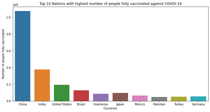
plt.figure(figsize=(12, 6))
sns.barplot(data=sorted_df[:10],x=sorted_df.index[:10],y='people_fully_vaccinated')
plt.title('Top 10 Nations with highest number of people fully vaccinated against COVID-19')
plt.ylabel('Number of people fully vaccinated')
plt.xlabel('Countries')
Text(0.5, 0, 'Countries')
sorted_df['people_not_fully_vaccinated_per_hundred'] = 100-sorted_df['people_fully_vaccinated_per_hundred']
# estimate population
sorted_df['population'] = sorted_df['people_fully_vaccinated']/sorted_df['people_fully_vaccinated_per_hundred']
sorted_df.head()
| iso_code | date | total_vaccinations | people_vaccinated | people_fully_vaccinated | total_boosters | daily_vaccinations_raw | daily_vaccinations | total_vaccinations_per_hundred | people_vaccinated_per_hundred | people_fully_vaccinated_per_hundred | total_boosters_per_hundred | daily_vaccinations_per_million | daily_people_vaccinated | daily_people_vaccinated_per_hundred | people_not_fully_vaccinated_per_hundred | population | |
|---|---|---|---|---|---|---|---|---|---|---|---|---|---|---|---|---|---|
| location | |||||||||||||||||
| China | CHN | 2021-11-15 | 2.396045e+09 | 1.185237e+09 | 1.073845e+09 | 49440000.0 | 24741000.0 | 22424286.0 | 165.91 | 82.07 | 74.35 | 3.42 | 15527.0 | 5850649.0 | 0.405 | 25.65 | 1.444311e+07 |
| India | IND | 2021-11-16 | 1.133688e+09 | 7.560527e+08 | 3.776355e+08 | NaN | 18627269.0 | 10037995.0 | 81.36 | 54.26 | 27.10 | NaN | 7204.0 | 6785334.0 | 0.487 | 72.90 | 1.393489e+07 |
| United States | USA | 2021-11-16 | 4.433742e+08 | 2.276919e+08 | 1.939638e+08 | 30651760.0 | 4516889.0 | 3498728.0 | 131.83 | 67.70 | 57.67 | 9.11 | 10403.0 | 2028734.0 | 0.603 | 42.33 | 3.363340e+06 |
| Brazil | BRA | 2021-11-16 | 2.971040e+08 | 1.623420e+08 | 1.279980e+08 | 11814702.0 | 11231782.0 | 2595170.0 | 138.84 | 75.86 | 59.81 | 5.52 | 12127.0 | 1394879.0 | 0.652 | 40.19 | 2.140078e+06 |
| Indonesia | IDN | 2021-11-16 | 2.166636e+08 | 1.312929e+08 | 8.537068e+07 | NaN | 3087420.0 | 1901294.0 | 78.40 | 47.51 | 30.89 | NaN | 6880.0 | 1160342.0 | 0.420 | 69.11 | 2.763700e+06 |
plot_df = sorted_df[['people_fully_vaccinated_per_hundred', 'people_not_fully_vaccinated_per_hundred','population']]
plot_df['location'] = plot_df.index
plot_df = plot_df.sort_values('population', ascending=False)
plot_df
| people_fully_vaccinated_per_hundred | people_not_fully_vaccinated_per_hundred | population | location | |
|---|---|---|---|---|
| location | ||||
| Burundi | 0.00 | 100.00 | inf | Burundi |
| China | 74.35 | 25.65 | 1.444311e+07 | China |
| India | 27.10 | 72.90 | 1.393489e+07 | India |
| United States | 57.67 | 42.33 | 3.363340e+06 | United States |
| Indonesia | 30.89 | 69.11 | 2.763700e+06 | Indonesia |
| ... | ... | ... | ... | ... |
| Montserrat | 28.45 | 71.55 | 4.980668e+01 | Montserrat |
| Falkland Islands | 50.31 | 49.69 | 3.528126e+01 | Falkland Islands |
| Niue | 71.25 | 28.75 | 1.614035e+01 | Niue |
| Tokelau | 70.76 | 29.24 | 1.368005e+01 | Tokelau |
| Pitcairn | 100.00 | 0.00 | 4.700000e-01 | Pitcairn |
217 rows × 4 columns
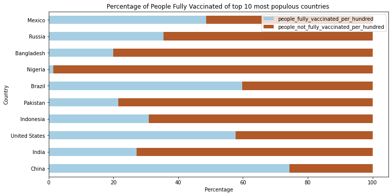
plot_df = plot_df[1:11].drop('population', 1) # drop first row
ax = plot_df.plot(figsize = (12, 6),
x = 'location',
kind = 'barh',
stacked = True,
title = 'Percentage of People Fully Vaccinated of top 10 most populous countries ',
mark_right = True,
colormap='Paired')
ax.set_xlabel("Percentage")
ax.set_ylabel("Country")
Text(0, 0.5, 'Country')
# Covid deaths over the time period
fig = px.choropleth(data_frame=sorted_df, locations='iso_code',
color='people_fully_vaccinated_per_hundred')
fig.show()
Vaccination in Germany over time
df_de = df[df['iso_code'] == 'DEU'].sort_values('date')
df_de.head()
| location | iso_code | date | total_vaccinations | people_vaccinated | people_fully_vaccinated | total_boosters | daily_vaccinations_raw | daily_vaccinations | total_vaccinations_per_hundred | people_vaccinated_per_hundred | people_fully_vaccinated_per_hundred | total_boosters_per_hundred | daily_vaccinations_per_million | daily_people_vaccinated | daily_people_vaccinated_per_hundred | |
|---|---|---|---|---|---|---|---|---|---|---|---|---|---|---|---|---|
| 20817 | Germany | DEU | 2020-12-27 | 24355.0 | 24344.0 | 11.0 | NaN | NaN | NaN | 0.03 | 0.03 | 0.0 | NaN | NaN | NaN | NaN |
| 20818 | Germany | DEU | 2020-12-28 | 42459.0 | 42384.0 | 75.0 | NaN | 18104.0 | 18104.0 | 0.05 | 0.05 | 0.0 | NaN | 216.0 | 18040.0 | 0.022 |
| 20819 | Germany | DEU | 2020-12-29 | 93182.0 | 92454.0 | 727.0 | 1.0 | 50723.0 | 34414.0 | 0.11 | 0.11 | 0.0 | 0.0 | 410.0 | 34055.0 | 0.041 |
| 20820 | Germany | DEU | 2020-12-30 | 157311.0 | 156551.0 | 759.0 | 1.0 | 64129.0 | 44319.0 | 0.19 | 0.19 | 0.0 | 0.0 | 528.0 | 44069.0 | 0.053 |
| 20821 | Germany | DEU | 2020-12-31 | 207320.0 | 206473.0 | 846.0 | 1.0 | 50009.0 | 45741.0 | 0.25 | 0.25 | 0.0 | 0.0 | 545.0 | 45532.0 | 0.054 |
fig=make_subplots()
fig.add_trace(go.Scatter(x=df_de['date'],y=df_de['people_vaccinated_per_hundred'],name="percentage_people_vaccinated"))
fig.add_trace(go.Scatter(x=df_de['date'],y=df_de['people_fully_vaccinated_per_hundred'],name="percentage_people_fully_vaccinated"))
fig.update_layout(autosize=False,width=900,height=600,title_text="Vaccination in Germany")
fig.update_xaxes(title_text="Date")
fig.update_yaxes(title_text="Number",secondary_y=False)
fig.show()
Nun sind ungefähr 67,7% der deutschen Gesamtbevölkerung vollständig geimpft (17.11.2021)
Covid Death
! kaggle datasets download -d dhruvildave/covid19-deaths-dataset
! mkdir train
! unzip covid19-deaths-dataset.zip -d train
mkdir: cannot create directory ‘train’: File exists
Archive: covid19-deaths-dataset.zip
inflating: train/all_weekly_excess_deaths.csv
inflating: train/us-counties.csv
EDA
import numpy as np
import pandas as pd
import matplotlib.pyplot as plt
import seaborn as sns
import plotly.express as px
import plotly.graph_objects as go
from plotly.subplots import make_subplots
import warnings
from collections import Counter
import operator
Data Statistics Exploration
df = pd.read_csv("train/all_weekly_excess_deaths.csv")
df.head()
| country | region | region_code | start_date | end_date | days | year | week | population | total_deaths | covid_deaths | expected_deaths | excess_deaths | non_covid_deaths | covid_deaths_per_100k | excess_deaths_per_100k | excess_deaths_pct_change | |
|---|---|---|---|---|---|---|---|---|---|---|---|---|---|---|---|---|---|
| 0 | Australia | Australia | 0 | 2019-12-30 | 2020-01-05 | 7 | 2020 | 1 | 25788217 | 2510.0 | 0.0 | 2569.892790 | -59.892790 | 2510.0 | 0.0 | -0.232249 | -0.023306 |
| 1 | Australia | Australia | 0 | 2020-01-06 | 2020-01-12 | 7 | 2020 | 2 | 25788217 | 2523.0 | 0.0 | 2565.059457 | -42.059457 | 2523.0 | 0.0 | -0.163096 | -0.016397 |
| 2 | Australia | Australia | 0 | 2020-01-13 | 2020-01-19 | 7 | 2020 | 3 | 25788217 | 2516.0 | 0.0 | 2543.559457 | -27.559457 | 2516.0 | 0.0 | -0.106868 | -0.010835 |
| 3 | Australia | Australia | 0 | 2020-01-20 | 2020-01-26 | 7 | 2020 | 4 | 25788217 | 2619.0 | 0.0 | 2544.892790 | 74.107210 | 2619.0 | 0.0 | 0.287368 | 0.029120 |
| 4 | Australia | Australia | 0 | 2020-01-27 | 2020-02-02 | 7 | 2020 | 5 | 25788217 | 2522.0 | 0.0 | 2532.392790 | -10.392790 | 2522.0 | 0.0 | -0.040301 | -0.004104 |
df.info() # no missing values found
<class 'pandas.core.frame.DataFrame'>
RangeIndex: 8630 entries, 0 to 8629
Data columns (total 17 columns):
# Column Non-Null Count Dtype
--- ------ -------------- -----
0 country 8630 non-null object
1 region 8630 non-null object
2 region_code 8630 non-null object
3 start_date 8630 non-null object
4 end_date 8630 non-null object
5 days 8630 non-null int64
6 year 8630 non-null int64
7 week 8630 non-null int64
8 population 8630 non-null int64
9 total_deaths 8630 non-null float64
10 covid_deaths 8630 non-null float64
11 expected_deaths 8630 non-null float64
12 excess_deaths 8630 non-null float64
13 non_covid_deaths 8630 non-null float64
14 covid_deaths_per_100k 8630 non-null float64
15 excess_deaths_per_100k 8630 non-null float64
16 excess_deaths_pct_change 8630 non-null float64
dtypes: float64(8), int64(4), object(5)
memory usage: 1.1+ MB
df.describe()
| days | year | week | population | total_deaths | covid_deaths | expected_deaths | excess_deaths | non_covid_deaths | covid_deaths_per_100k | excess_deaths_per_100k | excess_deaths_pct_change | |
|---|---|---|---|---|---|---|---|---|---|---|---|---|
| count | 8630.000000 | 8630.000000 | 8630.000000 | 8.630000e+03 | 8630.000000 | 8630.000000 | 8630.000000 | 8630.000000 | 8630.000000 | 8630.000000 | 8630.000000 | 8630.000000 |
| mean | 6.999421 | 2020.398378 | 23.668366 | 1.814569e+07 | 3344.657451 | 357.936443 | 2861.936587 | 482.720864 | 2986.721008 | 1.865979 | 2.406849 | 0.147073 |
| std | 0.053823 | 0.489592 | 14.283964 | 3.830643e+07 | 7431.723548 | 1179.567170 | 6252.342704 | 1727.999538 | 6564.975068 | 2.861617 | 3.884268 | 0.248748 |
| min | 2.000000 | 2020.000000 | 1.000000 | 3.433600e+05 | 28.000000 | -1625.000000 | 36.958708 | -3900.712360 | -1740.000000 | -8.803323 | -8.774060 | -0.450265 |
| 25% | 7.000000 | 2020.000000 | 12.000000 | 2.689862e+06 | 550.000000 | 4.000000 | 494.844756 | 3.459340 | 503.000000 | 0.113038 | 0.109435 | 0.006566 |
| 50% | 7.000000 | 2020.000000 | 23.000000 | 6.732219e+06 | 1248.000000 | 44.000000 | 1116.339077 | 68.225000 | 1123.000000 | 0.815235 | 1.424369 | 0.085771 |
| 75% | 7.000000 | 2021.000000 | 34.000000 | 1.717309e+07 | 2679.000000 | 210.000000 | 2367.852564 | 281.271795 | 2404.750000 | 2.356389 | 3.432663 | 0.206313 |
| max | 7.000000 | 2021.000000 | 53.000000 | 3.283005e+08 | 87342.000000 | 23481.000000 | 62621.817308 | 27935.009878 | 70474.000000 | 43.366504 | 48.776239 | 3.759663 |
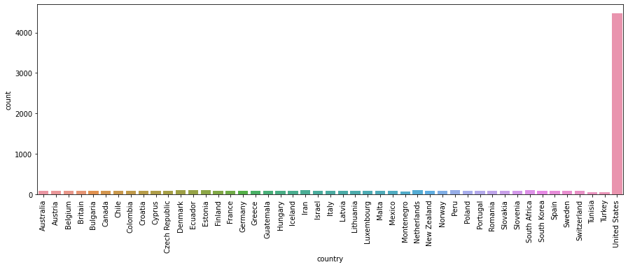
# we plot numbe of entries in the dataset
fig, ax = plt.subplots(1,1,figsize=(15,5))
sns.countplot(data=df,x='country',ax=ax)
plt.xticks(rotation=90)
plt.show()
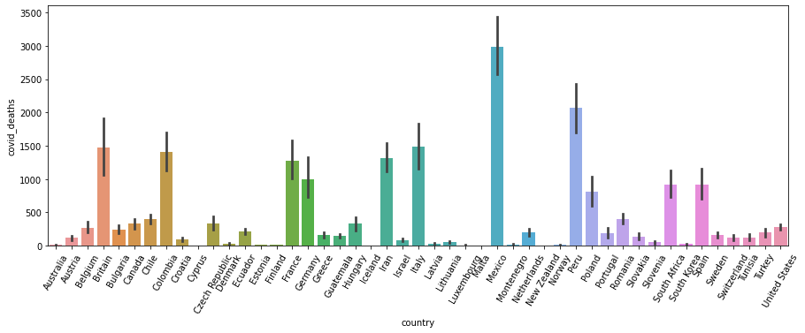
# plot the total number of death cases
fig,ax = plt.subplots(1,1,figsize=(15,5))
sns.barplot(data=df,x='country',y='covid_deaths')
plt.xticks(rotation=60)
plt.show()
# plot the percentage of COVID death cases
fig,ax =plt.subplots(1,1,figsize=(15,5))
df["covid_death_percent"] = df["covid_deaths"]/df["total_deaths"] * 100
sns.barplot(data=df,x='country',y='covid_death_percent')
plt.xticks(rotation=90)
plt.show()
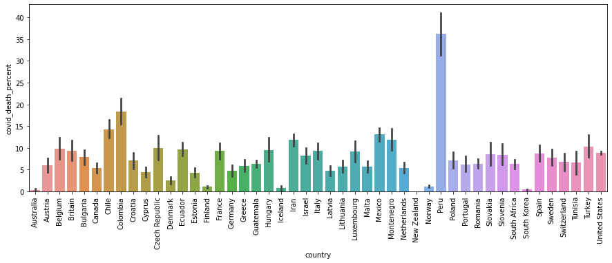
Mexico has the highest number of Covid death and Peru has the highest perentage of Covid death
# Covid deaths over the time period
fig = px.choropleth(data_frame=df, locations='country',
locationmode='country names', color='covid_deaths',
animation_frame='end_date')
fig.show()
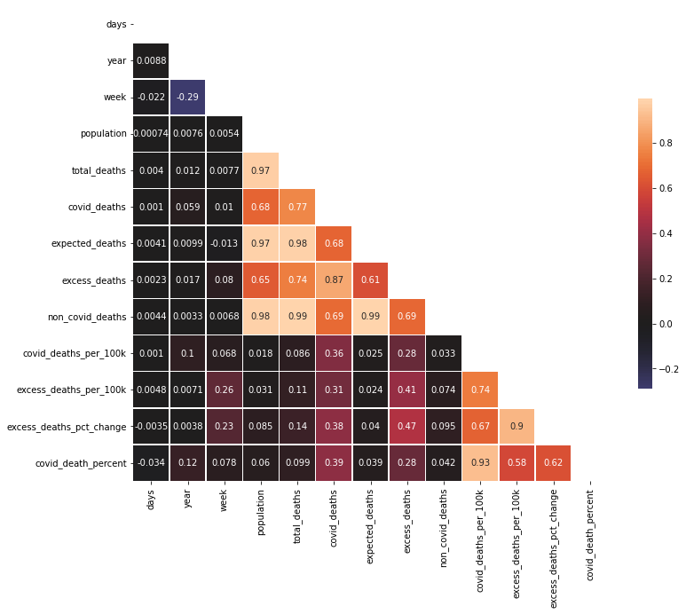
corr = df.corr()
mask = np.zeros_like(corr)
mask[np.triu_indices_from(mask)] = True
plt.figure(figsize=(12,12))
sns.heatmap(corr, mask=mask, center=0, annot=True,
square=True, linewidths=.5, cbar_kws={"shrink": .5})
plt.show()
# death case over 2 years
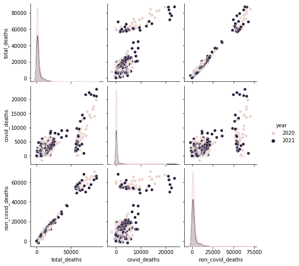
df['non-covid death'] = df['total_deaths'] -df['covid_deaths']
sns.pairplot(df, vars = ['total_deaths', 'covid_deaths', 'non_covid_deaths'], hue = 'year')
<seaborn.axisgrid.PairGrid at 0x7fb9d9d3e190>
Explore Covid Death Data in Germany
data_de = df[df['region']=='Germany']
data_de.head()
| country | region | region_code | start_date | end_date | days | year | week | population | total_deaths | covid_deaths | expected_deaths | excess_deaths | non_covid_deaths | covid_deaths_per_100k | excess_deaths_per_100k | excess_deaths_pct_change | covid_death_percent | |
|---|---|---|---|---|---|---|---|---|---|---|---|---|---|---|---|---|---|---|
| 1463 | Germany | Germany | 0 | 2019-12-30 | 2020-01-05 | 7 | 2020 | 1 | 83900471 | 18883.0 | 0.0 | 19399.361891 | -516.361891 | 18883.0 | 0.0 | -0.615446 | -0.026617 | 0.0 |
| 1464 | Germany | Germany | 0 | 2020-01-06 | 2020-01-12 | 7 | 2020 | 2 | 83900471 | 19408.0 | 0.0 | 19754.528558 | -346.528558 | 19408.0 | 0.0 | -0.413023 | -0.017542 | 0.0 |
| 1465 | Germany | Germany | 0 | 2020-01-13 | 2020-01-19 | 7 | 2020 | 3 | 83900471 | 18953.0 | 0.0 | 19675.528558 | -722.528558 | 18953.0 | 0.0 | -0.861173 | -0.036722 | 0.0 |
| 1466 | Germany | Germany | 0 | 2020-01-20 | 2020-01-26 | 7 | 2020 | 4 | 83900471 | 18827.0 | 0.0 | 19837.695225 | -1010.695225 | 18827.0 | 0.0 | -1.204636 | -0.050948 | 0.0 |
| 1467 | Germany | Germany | 0 | 2020-01-27 | 2020-02-02 | 7 | 2020 | 5 | 83900471 | 19774.0 | 0.0 | 20563.361891 | -789.361891 | 19774.0 | 0.0 | -0.940831 | -0.038387 | 0.0 |
fig=make_subplots()
fig.add_trace(go.Scatter(x=data_de['start_date'],y=data_de['total_deaths'],name="total_deaths"))
fig.add_trace(go.Scatter(x=data_de['start_date'],y=data_de['covid_deaths'],name="covid_deaths"))
fig.add_trace(go.Scatter(x=data_de['start_date'],y=data_de['expected_deaths'],name="expected_deaths"))
fig.add_trace(go.Scatter(x=data_de['start_date'],y=data_de['excess_deaths'],name="excess_deaths"))
fig.update_layout(autosize=False,width=900,height=600,title_text="Covid Deaths in Germany")
fig.update_xaxes(title_text="Date")
fig.update_yaxes(title_text="Number",secondary_y=False)
fig.show()
We see that excess death is close to covid death
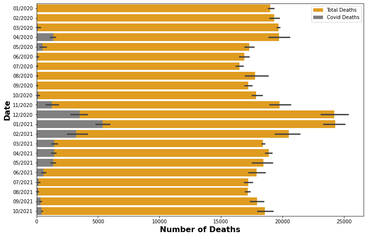
plt.figure(figsize=(12,8))
df_temp = data_de['end_date'].str.split('-', expand=True)[[1,0]]
data_de['date'] = df_temp[1] + '/' + df_temp[0]
sns.barplot(data=data_de, x='total_deaths', y='date', color='orange', label='Total Deaths')
sns.barplot(data=data_de, x='covid_deaths', y='date', color='grey', label='Covid Deaths')
plt.xlabel(xlabel = 'Number of Deaths',fontsize=16, fontweight='bold')
plt.ylabel(ylabel = 'Date',fontsize=16, fontweight='bold')
plt.legend()
plt.show()